|
by ARNE BATTERMANN
This section describes the processes listed below:
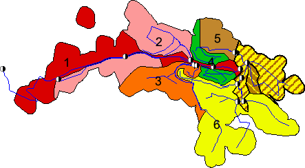
The zoning of the distribution system Judayta changes from summer to winter time. While Judayta is divided into six zones from April to November (figure 29), the network is operated with four zones in the winter months shown in figure 30.
The different zonings in summer and winter should allow an adjustment to different demand patterns. In fact, the bigger winter zones reduce the pumping head a little bit - higher friction losses are the reason.
During summertime each of the zones 2, 3, 4, 5 and 6 are supplied over 12 hours. Zone 1 is supplied over the whole interval. Missing separation of zones is recognizable between zone 5 and 6. Hazy zones are hatched yellow and brown. The total duration of supply is 60 hours.
The distribution zones are separated with the operation of 16 valves in the village. One of these valves is out of order currently - it is opened all the time because the gate has been taken out.
The first zone is supplied over 60 hours. The second zone is supplied over the first 24 hours and the third zone between the 24th and 48th hour. The fourth zone is supplied over the last 10 hours. As mentioned above a clear separation of zones does not exist. The yellow-brown hatched areas between third and fourth zone are supplied over the last 34 hours.
This schedule may vary depending on necessities. During the logging campaign the scheduled timetable was basically valid.
For the integration of the COBOSS data (section 3.3) the data needs to be checked (section 8.2.1). Afterwards the consumption of subscribers in Judayta has to be integrated into the GIS. The workflow is described in section 8.2.2.
The delivered COBOSS data consists of 4 meter-reading cycles from January 2000 to October 2000. Two of the cycles represent winter consumption and the other two cycles the summer consumption. In table 8 the billed consumption of Judayta village cycle is shown for the mentioned reading cycles.
Judayta has 1212 registered subscribers. In [11] based on the hydraulic analysis study of SOGREAH (Chapter 3.1) 8.5 persons are assigned to one subscriber in the greater area around Irbid.
| |||||||||||||||||||||||||||||||||||
The values for the consumption worked out in table 8
are within the ranges in Irbid of 180 - 650
![]() and
a resulting per capita consumption of 22 - 76
and
a resulting per capita consumption of 22 - 76
![]() published
in [11].
published
in [11].
With a measured well production of app. 80
![]() and
an estimated back flow of 10% (chapter 3.9) at
the well production an estimated average quantity of app. 70
and
an estimated back flow of 10% (chapter 3.9) at
the well production an estimated average quantity of app. 70
![]() is
pumped to Judayta over 60 hours of supply:
is
pumped to Judayta over 60 hours of supply:
Quantity of water pumped to Judayta during one full supply period (logging campaign / winter 2001):
70![]() . 60h = 4200m3
. 60h = 4200m3
Difference between pumped quantity and average billed consumption during winter months in Judayta :
4200m3 - 2542m3 = 1658m3
![]() . 100 = 39.5%
. 100 = 39.5%
The result is an UFW figure of app. 40%. This result reflects the expected value according to the tendency of decreasing UFW during the last ten years in Irbid and Jerash Governorate [11].
In order to integrate the COBOSS data into the hydraulic model a sequence of operations has to take place.
The link between the tabulated COBOSS and the GIS data is the primary key (PK) as used by the DLS. The PK is a unique ID for every single parcel in Jordan. Before the two data source can actually be linked, the following clean-up process has to take place:
The spatial data may contain duplicate primary keys for some reasons. For example, if a house is shown on the parcel, house and parcel will be represented by two records in the database, sharing the same PK. In order to prevent the billed consumption from being duplicated, all GIS records sharing the same PK have to be merged into one record.
There are also duplicated primary keys in the COBOSS data. Every time a parcel is home to more than one subscriber such duplications happen. As for the GIS data, it is necessary to merge all records sharing one PK into one. Additional, the billed consumption has to be summarized in order not to get lost during the linking process.
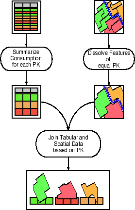
The steps required for joining COBOSS and GIS data are shown in figure 31.
After summary of equal PKs and concurrent creation of total consumption for each primary key the tabular and spatial data can be joined based on the PK. Now the spatial records in the GIS are completed with the characteristic consumption and the next operation in the sequence for integrating the consumption into the hydraulic model can start.
The ArcView functions used have been particularly the 'Summarize' function for the tabular data and the 'Geoprocessing Wizard - Dissolve features based on an attribute' for the spatial data.
As only the parcels with actual consumption are of interest, these are selected with a query. The following steps will only use these consumer parcels.
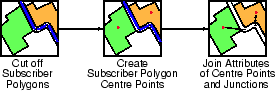
Within the next operation shown in figure 32, points shall be created, which contain the specific consumption of its polygons and the attributes of the nearest junction. Afterwards points are created in the centre of each polygon.
These points locate the house tanks. Therefore each centre point has to have the information to which junction of the water network it shall be connected, because house connections will be created between the tanks and the nearest junctions. By joining the attributes of the nearest junction with the consumption in the new generated centre points each centre point has the ID of that Junction and a relation is created.
In this operation the 'DC Conversion Extension' and the 'Geoprocessing Wizard are used. Centre points are created over 'DC Conversion Extension'13, while the 'Geoprocessing Wizard - Spatial Join' function is used to join the attributes of junctions with the attributes of the nearest centre points.
The final operation to create tanks with a realistic size at realistic locations is presented in figure 33. To generalize the tertiary water network the centre points are grouped first. This grouping is possible by creating multi-points of the centre points in the GIS. Multipoint data consists of several points that share the attributes, whereas for point themes, every point has a separate set of attributes.
Afterwards single points are generated by calculating the centre point of the created group. These single points represent the house tanks.
For this operation the 'Geoprocessing Wizard - dissolve features based on an attribute' has been used to generate a multi point theme. The single points are created by using 'DC Conversion Extension - create points from multi points'.
As the rest of the nodes in the water distribution network, the tanks need elevations. The elevations can be assigned from the DEM by using `DC Conversion Extension - assign point attribute from grid`.
The creation of 'house connections' is the final step for integrating the generalized house tanks into the water distribution network. House connections are generated between the tank and the nearest junction. The decisive step is already done before and shown in figure 32.
Attributes are taken over from the nearest junction and integrated into the centre point theme. Afterwards each tank has the same ID as the nearest junction. The DC Water Design Extension (appendix 11) is generating pipelines between the tanks and junctions into the pipe theme.
The major part of the work in the GIS is done with the connection of tanks with the distribution network.
In the present section the steps necessary to create a hydraulic model out of the GIS. The Water Design Extension (appendix 11) serves as the interface between ArcView and EPANET several tables and rules (section 8.3.6) have to be integrated into the process of converting the GIS data into an EPANET import file.
Preparing a separated model of Judayta is described in section 8.3.1. The elements of the network are defined in section 8.3.2. EPANET is a complex tool with powerful capabilities, therefore adjustments have to be made for this particular hydraulic model (section 8.3.3). The integration of demand and leakage into the model is explained in the sections 8.3.4 and 8.3.5.
The isolation of Judayta in the GIS is necessary for creating an EPANET model of this single village. The Water Design Extension provides a function that minimizes the work to cut out the elements belonging to one distribution zone like Judayta. This function for cutting off so called bit-code zones is described in section 7.5.
Once the elements of the Judayta water network or any other village need to be defined with an attribute in each theme. This attribute consists of a particular value for each village of Al Koura (figure 24). This means that the network of each village can be cut out separately and elements that are shared with other models (e.g. the pumping station) are included.
The aim of this method is to automate the process of manually cutting out the villages after updating elements in the GIS (new pipes, new valves, etc.), while still allowing to work on one seamless network map.
For creating an EPANET model of Judayta the following network elements are necessary:
Junctions are connected by pipes. The demand of the junctions is set on 0 because in this approach consumption is implemented with the tanks.
Valves allow to define distribution zones in extended period simulations (section 8.3.6). Judayta consists of 16 valves. One of these valves is currently out of order. All the network valves are modeled as Shut-Off-Valves (SOV).
The operating pump during supply of Judayta has to be characterized. Important pump informations like power (section 12.5) and pump curve (section 12.15) are integrated over the attributes ``Power'' and ``Properties''. While power is implemented as a value in the pump theme, the pump curve is integrated as an extra table with x- and y-coordinates. The data in the ''properties''-field is a link and contains the name of the pump curve.
Tanks are integrated to model leakage and demand. To different types of tanks are used:
The leakage tanks are generated at each junction of the water distribution network. The limiting factor for leakage is not the tank size but the diameter of the connection pipe (section 8.3.5).
A reservoir is necessary at the pumping station to feed the pumps in the EPANET model. It is a simplification of the hydraulic model. The two wells, which are filling the storage tank in Judayta pumping station (figure 9) are not integrated in the hydraulic model. Instead a reservoir is chosen for supplying the operating horizontal pumps. This reservoir resembles the pumping station's storage tank which is filled by the submersible pumps.
The pipes are structured in three types. The following types are defined:
The operations in the GIS for creating house connection pipes are shown in section 8.2.2. The house connection pipes shall supply the generalized house tanks. 125 house connections do exist in Judayta. It has to be made sure that a back flow of water from the house tank (section 8.3.4) is not possible. This has to be defined in the pipes theme of the GIS (section 8.3.6).
Leakage tank pipes are generated between the leakage tanks and the nearest junction. The GIS operations for generating these pipes are equal to the operations for house connections (section 8.2.2). The present hydraulic analysis model of Judayta village features of 157 leakage pipes. Each pipe has a length of 2 metres. The diameter of the leakage pipe is the key for modeling leakage in this approach.
For running an EPANET model basic adjustments have to be fixed. They have to be defined over the following items:
The options table allows to choose the used head-loss formula (in this case Darcy-Weissbach), define flow units (litres per second). The number of trials for finding hydraulic solutions can be specified (section 12.11).
These adjustments are not of the priority like Options or Times. The scale can be determined for getting different kind of summaries, status or warning reports. The used adjustments are described in appendix 12 (section 12.12).
The hydraulic time step and the duration of simulation period have to be defined. The duration is set to 58 hours and a hydraulic time step of 5 minutes is chosen.
Next to these to adjustments further items have to be defined (section 12.13)
While classical models have a specified demand at each network junction, the described approach is based on tanks which are filling in dependency of the present pressure at the tank (section 7.3).
The creation of house tanks is shown in section 8.2.
For a better visualization of the development of pressure and demand in EPANET each tank is reduced in its height to one metre. Like this a pressure scale from 0.1 to 1.0 in EPANET can visualize the tank fill level during the simulation period. The tank volumes have to be converted. Each tank is of cylindrical shape with a varying diameter and a constant height of one metre:
with
d = Tank diameter
V= Volume of tank established in section 8.2.
The house tanks are supplied over the so-called ``house connection pipes''. The diameter of all the house connections was initially chosen with 25mm. This global diameter yields a mistake because the diameters for house connections vary in reality. To overcome the problem, the calibration script provides functionality to graduate 4 diameters based on the size of the house tank. Such a model represents the reality much better than a global diameter - it is still an error source, though.
To prevent a back flow of water out of the house tanks check valves are integrated into the model. Each house connection pipe is equipped with a check valve as shown in Figure 34.
For integrating the leakage into this approach of modeling intermittent supply, tanks are created at each junction of the water distribution network. The rate of leakage depends in this approach on the pipe length connected to the junction.
Two neighboured junctions are sharing the connected pipe with 50% of the length each. The diameter of the leakage pipe should depend on the resulting pipe length of the distribution network. Two approaches have been tried for integrating leakage into the model.
Repair statistics, published in [12], show that the majority (more than 90 %) of the repairs have been done on pipes of DN50 and smaller. The network of house connections is not integrated into the computed model and therefore this statistic can not be reflected. This is not the case in the represented hydraulic model. House connections are present, but they are unreal. Consumers are summarized and the real total length of house connections behind a particular tank of the hydraulic model can be much bigger than defined by the length of the modeled house connection.
l = ![]()
dL = f . l
Where dL is the diameter of the leakage pipe and f is a factor that has to be adjusted in the calibration process. The first choice of the multiplier depends on the resulting leakage pipe diameter. The pipe diameters covered a range from 0 to 30 mm in the calibration.
EPANET allows to create rules in extended period simulations. For example a valve control can be implemented which opens and closes valves for supplying particular zones.
During the process of creating a functional hydraulic model of intermittent supply in Judayta also several problems were faced. Irregularities in the computed pressure and flow during the first time intervals of the simulation period in EPANET happened. Pressure and flow changed in areas of the network, which have not been supplied yet. These model irregularities have been resolved.
The network valves are declared as 'shut off' valves. They are used for opening and closing the distribution zones during operation of the network (section 8.1). Adequately the valves are used in the hydraulic model shown in the following. The three zones of Judayta are analyzed with one EPANET model.
In this case the operation of the zones in the village shall be reflected by the settings of the valves. The status of the valves can be either 'open' or 'closed'. The so-called simple rule allows to change the setting of a valve at defined moments of the simulation period.
LINK V121 CLOSED AT TIME 00
LINK V101 CLOSED AT TIME 24
LINK V106 OPEN AT TIME 48
It might confuse that the first column contains ``link'' instead of ``valve''. Shut off valves are represented as a pipe in EPANET.
Similar to the valve rules in the paragraph above rules have to be implemented for pipes also. Due to irregularities in connection with pressure and flow in zones of no supply because of closed valves a rule is necessary. Pipes are closed during hours of no supply and opened during hours of supply.
LINK L2524 CLOSED AT TIME 0
LINK L2516 OPEN AT TIME 24
LINK L2617 CLOSED AT TIME 48
Each pipe (link) owns a dc_ID (section 6.2.4) listed in the second column of the rule above, followed by status of the pipe and the time of setting this status. The irregularities stopped after integrating these rules.
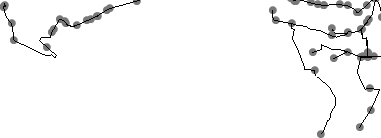
As mentioned in section 3.7 a logging campaign has been undertaken in Judayta. The flow was measured by two ultra-sonic flow meters 14. In addition, five pressure meters 15 have been used. The two flow meters stay at the same locations over the whole time of the supply interval. The locations of the pressure meters were changed over the supply time.
In the following an overview will be given for:
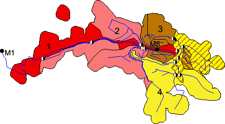
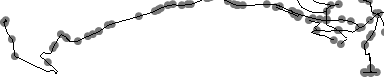
Flow measurements are intended at the pumping station and on the main pipe leading through the village in the centre of Judayta (figure 35). Problems occur with the flow meter at the pumping station (M1). The pressure readings are stopped after the first hours, because of pressure far above 30 bar.
The flow readings are not complete and error-prone due - partly due to turbulence and air inside of the pipe. At least 24 hours are not documented.
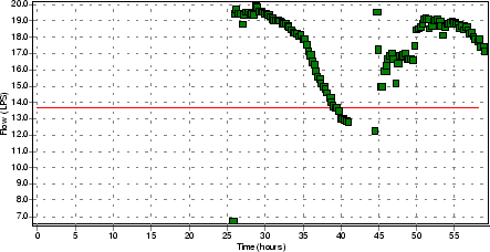
The readings of the second flow meter M5, shown in Figure 35, are realistic and used for calibrating the hydraulic model in EPANET.
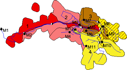
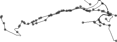
During the logging campaign 12 locations of Judayta (M1-M12) are measured depending on the operation of valves and the resulting supply zones (figure 36).
The pressure meters are installed at the domestic water meters.
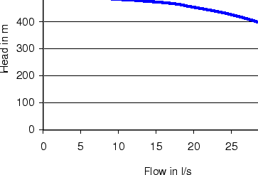
Because of unrealistic flow measurements behind the pumping station a characteristic pump curve for the operated pump cannot be obtained from the logging data. Pump measurements would have been necessary, but due to limited time these measurements have not been possible. In figure 37 the pump curve of the operated pump is shown. The data for this curve is delivered by the pump manufacturer [4].
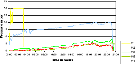
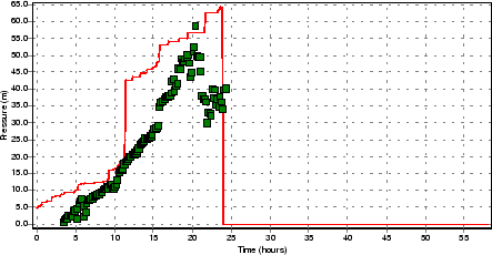
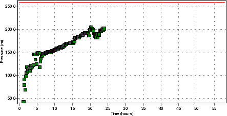
The tendencies of the pressure measurements are matching in all cases. During the first 24 hours the pressure is increasing slightly with an ascent of app. 4 metres per hour.
After 24 hours some valve settings are changed for supplying the second zone, this causes a pressure drop at the fixed ultra-sonic flow meter in the centre of Judayta.
The rapidly increasing pressure at M7 and M9 is noticeable. A reason might be the previous supply of the subscribers in the second zone next to the third zone. After 33 hours this demand seems to be satisfied and the pressure at M7 and M9 increases.
The flow starts at M5 24 hours after pumping started. The flow of
70
![]() is falling down to 45
is falling down to 45
![]() during
the following 16 hours.
during
the following 16 hours.
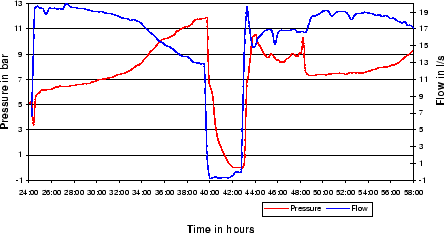
The reason for the decrease in flow at M5 (figure 40) and pressure at all measurement locations (figure 41) lies in a pump shut down. Three hours later the pump is switched on again. The pressure is rising nearly to the level before the shut down and is decreasing while the flow goes up until changing the valve settings are changed.
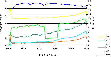
The flow during the last ten hours is constant at 65
![]() .
It is decreased slightly (0.5
.
It is decreased slightly (0.5
![]() ) while the
pressure is taking up by approximately 1
) while the
pressure is taking up by approximately 1
![]() .
.
The pressure at M11 drops for 1.5 hours in the middle of the last supply period. A reason could be a large consumer, located downstream on the same pipe. The steep incline in pressure after 1.5 hours can be a sign that the consumer's demand is fulfilled. The pressure measurements are fitting together and are reliable. They are reflecting the elevation differences of the locations quite good.
Except for the measurements at Logger M1 (figure 35) all measurements are of value for a model calibration. The supply interruption for 3 hours during the second day will cause difficulties in calibrating the model, because the pressure drop and the development of pressure and flow after this event are difficult to model and have therefore been disregarded.
A summary of all measurements is given in appendix 17.
On the basis of the measurements presented in section 8.4 the calibration of the EPANET model can start. In the following the steps towards calibrating the model are explained. Section 8.5.1 describes the preparation of the calibration files. The different operations and changes for reaching a better conformity of the computed and measured values are following in section 8.5.2. The results of calibrating the model with the final values of the themes are listed in section 8.5.3.
This section describes how to integrate the results of the logging
campaign into the hydraulic model. Two ASCII files have
to be generated consisting of flow and pressure measurements. The
structure of the files is easy and shown in the following examples.
The calibration file for the flow consists of the location of the
measurement, the time in hours and the measurement of flow in
![]() .
.
J2410 25:45 6.688055556
J2410 26:00 19.4225
J2410 26:15 19.69444444
The calibration file above consists of the measurements at M5 (figure 35) only. The measurements of the logger at location M1 are unreliable and useless for a calibration. The calibration file consists of 120 records in intervals of 15 minutes and reflects the flow in figure 40.
The pressure calibration file - which is structured in a similar way - is shown with the following example:
J2429 1:05 42.72
J2429 1:15 91.47
J2429 1:25 79.49
The pressure-calibration file consists of location, time and pressure
measurement in m. Measurements of all locations are listed sequentially.
Altogether ![]() 1650 pressure measurements in intervals
of 5 minutes at 12 locations of the distribution network can be used
for calibrating the hydraulic model.
1650 pressure measurements in intervals
of 5 minutes at 12 locations of the distribution network can be used
for calibrating the hydraulic model.
Before running a calibration in EPANET some irregular values have to be eliminated. In the beginning and end of the pressure and flow measurements values exist, which should not be used for a calibration. Zones have been closed already or the measurements are distorted by air in the filling/emptying network.
An improvement of calibration results, which are generated in EPANET has been managed by changing attributes of the pipe, pump and tank themes. The following attribute values have been varied in the calibration process:
After creating an import file for EPANET over the DC Water Design Extension the calibration files (section 8.5.1) have to be loaded into the EPANET import file and a ``Run'' of the model has to be started. With this run EPANET is calculating the development of pressure, flow, etc. during the defined simulation period. The comparison of the computed and measured values for flow and pressure can be illustrated as a graph showing the mistake of all locations or as graph for each measurement location. In reliance on the development of pressure and flow at the different locations further variations in ArcView have to be done for improving the current calibration results.
Because of the complexity of variation and combination the achievements in approximating the computed model to measured values have been limited even if the tendencies were getting better and better. The support of the calibration process by genetic algorithms (section 7.6.1) eased the process. Additionally different classes of house connections could be applied in a graduated manner.
The winter time supply periods could be summarized as follows:
Through the calibration process the model quality improved. The listed parameters in table 9 represent the best calibration of the model. They are the result of the calibration process. All multipliers are described in section 7.6. First estimations of a roughness between 1.5 and 2 are confirmed by the genetic algorithms.
|
Figure 42 depicts an example of the how the solutions improve during the Genetic Algorithm calibration process as described in section 7.6. Smaller fitness represent better solutions.
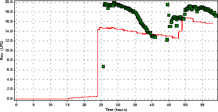
In figure 43 the computed flow is compared
to the measured flow at M5 (figure 35). During
the first day no flow is happening because the zone behind the logger
has been closed. A maximum difference between measured and computed
values of 5
![]() is given in the second zone. During
supply of the third zone the computed values are lying close to the
measurements.
is given in the second zone. During
supply of the third zone the computed values are lying close to the
measurements.
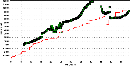
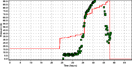
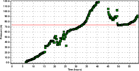
The pressure measurement at M5 between hour 6 and 42 is fitting with
the computed model in the tendency (figure 44).
The computed values differ approximately 5 - 20 m from the measured
values during the first day. With the opened zone behind the location
M5 and after 24 h the difference between model and measurement is
increasing. After 42 hours a gap of calibration measurements is noticeable.
Due to high pressure at the pumping station the operating pump has
been stopped for 4 hours. This was not be modeled in EPANET. The drop
of measurement data is deleted in the calibration file to avoid mistakes
as mentioned in section 8.5.1.
The consequence on the stopped pump is a complete pressure loss. After the pump operation starts again the pressure recovers on the computed flow level and increases similarly to the computed pressure.
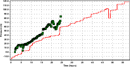
Figure 45 is representing the location M3 (shown in figure 36). The measured pressure is close to the computed model and the tendency is good.
A reason for the differences between computed and measured values shown in figure 44 and 45 could lay in the modeling of house tanks. The house tanks of the model are not equivalent to the house tanks hanging on a particular pipe in reality to 100%.
Some tank sizes of the model are too big, others are too small. This situation has an effect on the pressure of course. An even higher influence on the inaccuracy might stem from the distribution of leakage tanks in the network. Besides the elevations have an accuracy of app. 25 metres only. The DEM is cross-checked but differences have been ascertained. The measurement locations might lay up to 25 metres higher than fixed in the model.
Measurement locations in the village can not be reflected with the computed model easily. M4 and M7 are lying in densely populated areas. Despite the computed pressure is close to the measured values.
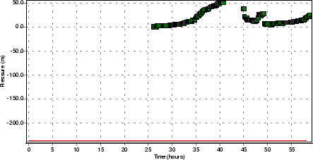
The constant positive pressure over the first 24 h shown in figure 47 is a problem of EPANET which is not designed to model intermittent supply. It happens in periods of empty pipes that EPANET shows pressures, even if the pipes are set on ``closed'' (section 8.3.6) because the zone is not supplied yet.
Nevertheless, the tendency of the model is fitting with the measurements. This is also shown in figure 47 representing location M7. Pressure level as well as tendencies are fitting between computed and measured values.
Figure 48 represents a pressure measurement at location M2. This location is the first on the way to Judayta and at the lowest point of all measurements. The computed pressure is much higher than the measured pressure. Possible reasons for the differences can be found for example in the accuracy of elevation. The mistake of 25m contour maps can be high due to the topography.
The necessity for creating hydraulic models of intermittent supply becomes clear by the comparison with traditional network analysis models. The tolerated inaccuracy of traditional models in areas of intermittent supply shall be demonstrated. In the following two traditional approaches to model the Judayta network are shown.
The first approach tries to simulate intermittent supply as far as possible with nodal demands. It models the different zones in separated hydraulic models (section 8.6.2). The demand of nodes depends on the operation of zones.
The second approach resembles the design of a continuous supply network. It is described in section 8.6.3. It consists of a one-zone model with a demand calculated directly out of the billed consumption. The operation of zones and the resulting change of demand are ignored.
The following parameters have to be adjusted in order to realize a traditional model with nodal demand:
The process is similar to the process described for the generation of the generalized household storage tanks.
Judayta can be divided into three zones while elements of the network have to be shared by zones (e.g. pumping station). In this context the important elements are the nodes (junctions). The junction theme gets a new attribute ``Duration'' in the Database.
After selecting the nodes, which are supplied over the first 24 h, the ``Duration'' for the selected elements is set on 24. All the other records stay set to 0. With selecting the next supply zone a duration of further 24 h is added to the nodes, which are supplied over the first day already:
existing value + 24
Like this nodes are defined which are supplied over 48, 24 and 0 h. With doing the same for the third zone the duration of supply is defined for each node of the network.
The roughness is defined with 1.63 mm for each pipe of the network (according to the previous calibration of the intermittent supply model; section 8.5.3, table 9).
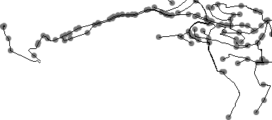
For the traditional model of Judayta described in section 8.6.2 the three zones shown in figure 49 have to be analyzed separately. Therefore the zones are cut out of the complete Judayta village data and presented as compact zones, which are supplied over different durations. The zones share elements for example the nodes and pipes between the pumping station and the western part of the village.
The EPANET models are shown in figure 49.
As mentioned above this model is used to model existing networks in intermittent supply areas usually.
In the following the calculation of nodal demand is described. Afterwards some examples of the computed model shall be shown with some figures.
The demand is implemented into the junction theme by re-calculating
the tank volume. Besides the demand has to be converted into
![]() .
A time simulation of continuous supply can be created on the basis
of this demand over 58
.
A time simulation of continuous supply can be created on the basis
of this demand over 58
![]() . This duration is chosen
for getting the opportunity of comparing results of the traditional
model with the approach of modeling intermittent supply.
. This duration is chosen
for getting the opportunity of comparing results of the traditional
model with the approach of modeling intermittent supply.
mQs = ![]() .
. ![]() . 1000 . mS . mL
. 1000 . mS . mL
with
mQs = Average demand in
![]()
Q3m = Consumption according to COBOSS during 3 month of
the year in
![]() with 14
with 14
![]()
hs = Time of supply according to operation of zones in h (24 h, 10 h)
ht, s = Total time of supply interval (58 h)
mL = Multiplier for considering Losses, estimated with 40%
mS = Peak factor
The peak factor is estimated as 1.4 [5]. The multiplier for considering losses is justified by measurements of back flow at the pumping station. UFW are estimated with 40% (section 5.1).
A calibration of the model is difficult because of its condition. The demand is not changing over the day because of house tanks in the distribution network. Therefore the system is static.
Figure 50 represents one of the best results of this model with a pressure of 7.4 bar. The computed pressure is close to an average value of the measurements. During the first supply interval the computed values of the other locations are of similar quality.
Especially during the supply of the third zone an extreme sub-pressure can be noticed at several locations (an example is given with figure 51). Warnings because of negative pressures are given by EPANET especially for this zone. In cases like this the pump size or parameters for increasing the power are changed usually. For reaching better results the pump speed has to be increased with 50%.
This essentially means that the respective models are broken.
This model consists of one zone as mentioned above. The demand is calculated directly out of the billed consumption without differentiation of nodes, which are supplied 24 h, 48 h or 58 h in reality. Each node is getting the demand in dependence on the specific consumption.
This approach is a simplification of the model described in section 8.6.2.
mQs = ![]() .
. ![]() . 1000 . mL . mS
. 1000 . mL . mS
mQs = Average demand in
![]()
Q3m = Billed consumption during 3 month of the year in
![]() with 14
with 14
![]()
mL = Multiplier for considering unaccounted-for water, estimated with 40%
mS = Peak factor, estimated at 40%.
The results are similar to the results of the first traditional model, presented in section 8.6.2.
The flow at M5 shown in figure 53 lies far below the measured values.
Also the computed pressure is to high and does not reflect the measurements as shown in figure 54.
Both traditional models have been analyzed. These models do not reflect intermittent supply. The point is that in reality tanks are filled in dependence on the present pressure. The traditional model ignores this by modeling the consumption as a nodal demand, which is pressure independent. As shown in figure 51 this continuous demand cannot be satisfied sometimes.
With the presented model of intermittent supply each node is getting that quantity of water, which is offered at a specific time and location. The quantity of water, which is running into a tank, depends on the pressure at this location and the pressure is influenced mainly by filling tanks and quantity of leakage below.
In addition to this mistake of traditional models in intermittent supply areas, the development of pressure, demand and flow over the time cannot be represented. However the present approach can deliver these informations as shown in section 8.5.3. Advantages of the intermittent supply model are listed in the following: